Single and Multi-Stage Valuation Multiples and Models

Single and Multi-Stage Valuation Multiples and Models

In Search of g

g In a Two-Stage Valuation Model

Single and Multi-Stage Valuation Multiples and Models

Enterprise multiples can be used as single-stage multiples in which the expected growth rate of the target firm’s income variable is constant, or more realistically, as a two-stage multiple in which the growth rate of the income is indicated at a specified rate during an explicit forecast period and then is held constant beyond that period of time, during a continuation period if you will. This is a more reasonable approach to valuation modeling of course.

Given that the outcome of a valuation model is intended to represent the firm’s Enterprise Value, we can think of a single-stage Enterprize Multiple as a type of valuation model. Suppose we’re using an EV/EBIT multiple such that 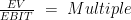$\frac{EV}{EBIT}\,\,=\,\, Multiple$ .

We can rearrange this to read $EV\,\,=\,\,Multiple\,\,x\,\,EBIT$ . In this context a single-stage multiple becomes a continuing value (terminal value) and follows the simple dividend yield equity valuation model $P_{0}\,\,=\,\,\frac{D_{1}}{WACC\,\,-\,\,g}$ .

If we substitute $EV$ for $P_{0}$ and $Multiple\,\,x\,\,EBIT$ for $\frac {D_{1}}{WACC\,\,-\,\,g}$ , and introduce time signatures to the variables the model reads $EV_{0}\,\,=\,\,Multiple\,\,x\,\,EBIT_{1}$ .

In this context the multiple is a forward market multiple (FMM) and informs the two-stage Forward Market Multiple Valuation Model, $Value _{FMM}\,\,=\,\,PV_{DCF}\,\,+PV_{CV}$ in which $CV_{FMM}\,\, =\,\,EBIT_{1}\,\, x\,\,\frac{EV_{0}}{EBIT_{0}}$ and $PV_{CV}\,\, = \,\, \frac{CV}{(1\,\,+\,\,WACC)^{t}}$ .

In search of g

EV is an observed value for the subject firms in this study as of a particular date and is the result of economic agents in the market setting bid and ask prices for marketable equity and debt securities; $EV\,\,=\,\,Market\,\, Value\,\, Equity\,\, Shares\,\, + \,\,Market\,\, Value\,\, Debt\,\, -\,\, Cash\,\,\&\,\, Equivalents$ . Similarly, EBIT is an observed value based on the accounting identity of $EBIT\,\,=\,\,Earnings\,\, before\,\, interest\,\,\&\,\,taxes$ . ROIC and WACC are simply derived values based on the identities 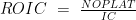$ROIC\,\,=\,\,\frac{NOPLAT}{IC}$ and $WACC\,=\,\frac{E}{V}\,R_{E}\, +\, \frac{P}{V}\,R_{P}\,+\,\frac{D}{V}\,R_{D}\,(1\,-\,T)$ , and $T\,\,=\,\,Average \,\,Tax\,\,Rate\,\,on\,\,EBIT$ and we can specify thier values with relative certainty.

With $EV,\,\, EBIT,\,\, ROIC,\,\, WACC,\,\, and\,\, T$ being known values, we can use the single-stage multiple 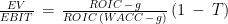$\frac {EV}{EBIT} \,= \,\frac{ROIC\, -\, g}{ROIC\,(WACC\,-\,g)}\,(1\,-\,T)$ to solve for $g$ and be confident that this $g$ is the rate of growth expected by the market for the subject firm…. and that happens to be very interesting.

As it turns out, when we solve for $g$ in this manner, each of the single-stage multiples in this study result in the same value of $g$ for a given firm as of a specified point in time.

g in a two-stage solution

Equally as interesting is the potential use of this $g$ in forming a target multiple. If investors are confident a firm’s management can increase $ROIC$ and/or reduce $WACC$ , we can then suppose these values interacted with the market inferred $g$ result in a target multiple in the form $\frac {EV}{EBIT} \,= \,\frac{ROIC\, -\, g}{ROIC\,(WACC\,-\,g)}\,(1\,-\,T)$ .

Finally, we can consider the use of these equations to solve for a firm’s long-run $g$ following some explicit period in a two-stage valuation model. Suppose we have explicit forecasts for Free Cash Flow $(FCF)$ for a three to five year period, after which we’re reticent to forecast a firm’s cash flow owing to the decrease in accuracy such forecasts tend to offer as time reaches forward. We can calculate the cash flow’s rate of growth during the explicit forecast period simply enough through the equation $\frac{FCF_{1}\,\,-\,\,FCF_{0}}{FCF_{0}}\,\,x\,\,100 \,\,=\,\, \% \Delta FCF$ , but we’re left to calculate the firm’s long-run: $\hat{g}$ . We can do this as follows:

Suppose $EV\,\,-\,\,PV_{DCF/FCF}\,\,=\,\,EV'$ and $EV'\,\,x\,\, (1\,\,+\,\,WACC)\,\,=\,\,\hat{EV}$ . We can then solve for $\hat{g}$ as follows:

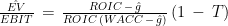$\frac{\hat{EV}}{EBIT}\,= \,\frac{ROIC\, -\, \hat{g}}{ROIC\,(WACC\,-\,\hat{g})}\,(1\,-\,T)$ and $\hat{g}\,\,=\,\frac{ROIC\,[(T'\, x\, EBIT)\,-\,(\hat{EV}\, x\, WACC)]}{(T'\,x\,EBIT)\,-\,(\hat{EV}\, x\, ROIC)}$ .

Once again, the $\hat{g}$ inferred through the use of a single-stage multiple, this time embedded in a two-stage valuation model, is consistent for a given firm at a specified point in time with the $\hat{g}$ calculated using other enterprise multiples. Only this time it’s not as interesting … by now we’ve come to expect it.